
Statistical comparison of samples with stat_tool#
This notebook illustates how to perform statistical tests and other analyses for comparing samples with stat_tool.comparison#
Load data sets (meri1.his to meri3.his)
[1]:
from openalea.stat_tool import (
    get_shared_data,
    Histogram,
    Vectors,
    VectorDistance,
    SelectVariable
)

from openalea.stat_tool.comparison import (
    ComparisonTest,
    Compare
)

from openalea.stat_tool.output import Plot

import numpy as np

meri1 = Histogram(get_shared_data("meri1.his"))
meri2 = Histogram(get_shared_data("meri2.his"))
meri3 = Histogram(get_shared_data("meri3.his"))
Running cmake --build & --install in /home/jdurand/devlp/Git/openalea/stat_tool/build
Running cmake --build & --install in /home/jdurand/devlp/Git/openalea/sequence_analysis/build
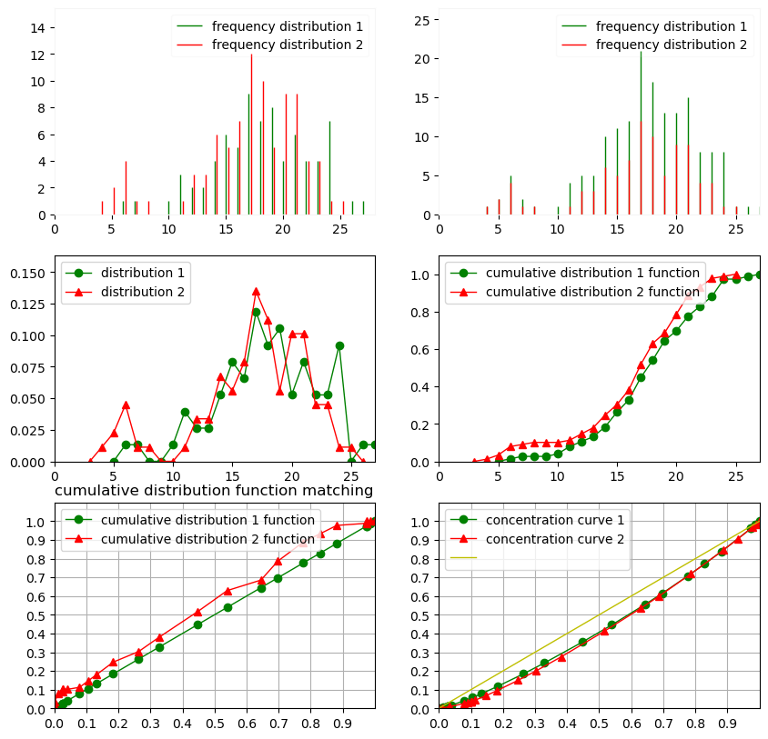
Exploratory analysis suggests that meri1 is globally larger than meri2
[2]:
Plot(meri1, meri2)
Statistical tests for comparing samples#
Student’s test for comparing means in Gaussian samples
Null hypothesis: sample 1 and sample 2 have the same means
[3]:
print(ComparisonTest("T", meri1, meri2))
two-sided t-test (162 degrees of freedom)
t-value: 1.87611   critical probability: 0.0624397
reference t-value: 1.97472   reference critical probability: 0.05
Alternative syntax, object-oriented:
[4]:
print(meri1.t_comparison(meri2))
two-sided t-test (162 degrees of freedom)
t-value: 1.87611   critical probability: 0.0624397
reference t-value: 1.97472   reference critical probability: 0.05
show sample means
[5]:
meri1.mean, meri2.mean
[5]:
(18.026315789473685, 16.707865168539325)
Wilcoxon-Mann-Whitney nonparametric test for comparing means in two samples
Null hypothesis: sample 1 and sample 2 have the same means.
[6]:
print(ComparisonTest("W", meri1, meri2))
two-sided Wilcoxon-Mann-Whitney test
standard normal value: 1.45438   critical probability: 0.145841
reference standard normal value: 1.95996   reference critical probability: 0.05
P(X1 < X2) = 0.400651   P(X1 = X2) = 0.0674157   P(X1 > X2) = 0.531934
[7]:
print(meri1.wmw_comparison(meri2))
two-sided Wilcoxon-Mann-Whitney test
standard normal value: 1.45438   critical probability: 0.145841
reference standard normal value: 1.95996   reference critical probability: 0.05
P(X1 < X2) = 0.400651   P(X1 = X2) = 0.0674157   P(X1 > X2) = 0.531934
Fisher’s test for comparing variances in Gaussian samples
Null hypothesis: sample 1 and sample 2 have the same variances.
[8]:
print(ComparisonTest("F", meri1, meri2))
F-test (88 degrees of freedom, 75 degrees of freedom)
F-value: 1.21097   critical probability: 0.19769
reference F-value: 1.44897   reference critical probability: 0.05
[9]:
print(meri1.f_comparison(meri2))
F-test (88 degrees of freedom, 75 degrees of freedom)
F-value: 1.21097   critical probability: 0.19769
reference F-value: 1.44897   reference critical probability: 0.05
show sample standard deviations
[10]:
np.sqrt(meri1.variance), np.sqrt(meri2.variance)
[10]:
(np.float64(4.295652637137618), np.float64(4.727103300963237))
Using Compare to compare more than 2 samples.#
This function prints each histogram separately, then using common rows and then prints dissimilarity measures between histograms. If the variables are numeric, an ANOVA is performed, as well as Fisher F-tests to compare variances.
The dissimilarity measure  between histograms
  and
and  , seen as arrays of relative frequencies, globally writes as:
between histograms and , seen as arrays of relative frequencies, globally writes as:
where
![d(h,h') = \sum\limits_k \sum\limits_{m > k} \rho(h[k] * h'[m] - h[m] * h'[k], m-k)](../_images/math/0ffd1fef587f8640a4b50e7fd6cb310168ca87e0.png)
![\rho(h[k] * h'[m] - h[m] * h'[k], m-k) =
\left\lbrace
\begin{array}{l}
|h[k] * h'[m] - h[m] * h'[k]| \textrm{ if the variable is ordinal, with} d(h,h') = -d(h',h) \\
h[k] * h'[m] - h[m] * h'[k] \textrm{ if the variable is symbolic, with } d(h,h') = d(h',h)\\
(m-k)(h[k] * h'[m] - h[m] * h'[k]) \textrm{ if the variable is numeric, with } d(h,h') = -d(h',h)\\
\end{array}
\right.](../_images/math/95792b0325b54d0661f454f2a4228264f8d0ce15.png)
[11]:
compare_numeric = Compare(meri1, meri2, meri3, "NUMERIC")
[12]:
print(compare_numeric)
frequency distribution 1 - sample size: 76
mean: 18.0263   median: 18   mode: 17
variance: 18.4526   standard deviation: 4.29565   lower quartile: 15   upper quartile: 21
coefficient of skewness: -0.370952   coefficient of kurtosis: -0.0181747
mean absolute deviation: 3.3705   coefficient of concentration: 0.132789
information: -207.685 (-2.7327)

frequency distribution 2 - sample size: 89
mean: 16.7079   median: 17   mode: 17
variance: 22.3455   standard deviation: 4.7271   lower quartile: 15   upper quartile: 20
coefficient of skewness: -0.977759   coefficient of kurtosis: 0.540819
mean absolute deviation: 3.55208   coefficient of concentration: 0.151923
information: -242.014 (-2.71926)

frequency distribution 3 - sample size: 120
mean: 12.9417   median: 14   mode: 15
variance: 14.9125   standard deviation: 3.86168   lower quartile: 10   upper quartile: 16
coefficient of skewness: -0.563081   coefficient of kurtosis: -0.649252
mean absolute deviation: 3.14347   coefficient of concentration: 0.165223
information: -307.094 (-2.55912)

   | frequency distribution 1 | frequency distribution 2 | frequency distribution 3 | cumulative distribution 1 function | cumulative distribution 2 function | cumulative distribution 3 function
 0   0   0   0          0          0          0
 1   0   0   0          0          0          0
 2   0   0   0          0          0          0
 3   0   0   0          0          0          0
 4   0   1   0          0   0.011236          0
 5   0   2   4          0  0.0337079  0.0333333
 6   1   4   8  0.0131579  0.0786517        0.1
 7   1   1   6  0.0263158  0.0898876       0.15
 8   0   1   5  0.0263158   0.101124   0.191667
 9   0   0   3  0.0263158   0.101124   0.216667
10   1   0   5  0.0394737   0.101124   0.258333
11   3   1   5  0.0789474    0.11236        0.3
12   2   3   5   0.105263   0.146067   0.341667
13   2   3  12   0.131579   0.179775   0.441667
14   4   6  15   0.184211   0.247191   0.566667
15   6   5  21   0.263158   0.303371   0.741667
16   5   7  14   0.328947   0.382022   0.858333
17   9  12   6   0.447368   0.516854   0.908333
18   7  10   7   0.539474   0.629213   0.966667
19   8   5   3   0.644737   0.685393   0.991667
20   4   9   0   0.697368   0.786517   0.991667
21   6   9   1   0.776316    0.88764          1
22   4   4       0.828947   0.932584
23   4   4       0.881579   0.977528
24   7   1       0.973684   0.988764
25   0   1       0.973684          1
26   1           0.986842
27   1                  1

dissimilarities between frequency distributions

            | frequency distribution 1 | frequency distribution 2 | frequency distribution 3
frequency distribution 1          0  -1.31845  -5.08465
frequency distribution 2    1.31845         0   -3.7662
frequency distribution 3    5.08465    3.7662         0

analysis of variance

source of variation | degrees of freedom | sum of squares | mean square
between samples    2  1400.11  700.055
within samples   282  5124.94  18.1736
total            284  6525.05  22.9755

F-test (2 degrees of freedom, 282 degrees of freedom)
F-value: 38.5205   critical probability: 1.62112e-15
reference F-value: 3.02778   reference critical probability: 0.05
reference F-value: 4.6812   reference critical probability: 0.01
An abbreviated version can be used for variable type: N, O or S.
[13]:
assert(compare_numeric == Compare(meri1, meri2, meri3, "N"))
[14]:
print(Compare(meri1, meri2, meri3, "ORDINAL"))
frequency distribution 1 - sample size: 76
mean: 18.0263   median: 18   mode: 17
variance: 18.4526   standard deviation: 4.29565   lower quartile: 15   upper quartile: 21
coefficient of skewness: -0.370952   coefficient of kurtosis: -0.0181747
mean absolute deviation: 3.3705   coefficient of concentration: 0.132789
information: -207.685 (-2.7327)

frequency distribution 2 - sample size: 89
mean: 16.7079   median: 17   mode: 17
variance: 22.3455   standard deviation: 4.7271   lower quartile: 15   upper quartile: 20
coefficient of skewness: -0.977759   coefficient of kurtosis: 0.540819
mean absolute deviation: 3.55208   coefficient of concentration: 0.151923
information: -242.014 (-2.71926)

frequency distribution 3 - sample size: 120
mean: 12.9417   median: 14   mode: 15
variance: 14.9125   standard deviation: 3.86168   lower quartile: 10   upper quartile: 16
coefficient of skewness: -0.563081   coefficient of kurtosis: -0.649252
mean absolute deviation: 3.14347   coefficient of concentration: 0.165223
information: -307.094 (-2.55912)

   | frequency distribution 1 | frequency distribution 2 | frequency distribution 3 | cumulative distribution 1 function | cumulative distribution 2 function | cumulative distribution 3 function
 0   0   0   0          0          0          0
 1   0   0   0          0          0          0
 2   0   0   0          0          0          0
 3   0   0   0          0          0          0
 4   0   1   0          0   0.011236          0
 5   0   2   4          0  0.0337079  0.0333333
 6   1   4   8  0.0131579  0.0786517        0.1
 7   1   1   6  0.0263158  0.0898876       0.15
 8   0   1   5  0.0263158   0.101124   0.191667
 9   0   0   3  0.0263158   0.101124   0.216667
10   1   0   5  0.0394737   0.101124   0.258333
11   3   1   5  0.0789474    0.11236        0.3
12   2   3   5   0.105263   0.146067   0.341667
13   2   3  12   0.131579   0.179775   0.441667
14   4   6  15   0.184211   0.247191   0.566667
15   6   5  21   0.263158   0.303371   0.741667
16   5   7  14   0.328947   0.382022   0.858333
17   9  12   6   0.447368   0.516854   0.908333
18   7  10   7   0.539474   0.629213   0.966667
19   8   5   3   0.644737   0.685393   0.991667
20   4   9   0   0.697368   0.786517   0.991667
21   6   9   1   0.776316    0.88764          1
22   4   4       0.828947   0.932584
23   4   4       0.881579   0.977528
24   7   1       0.973684   0.988764
25   0   1       0.973684          1
26   1           0.986842
27   1                  1

dissimilarities between frequency distributions

            | frequency distribution 1 | frequency distribution 2 | frequency distribution 3
frequency distribution 1           0  -0.131283  -0.629496
frequency distribution 2    0.131283          0  -0.520599
frequency distribution 3    0.629496   0.520599          0

Kruskal-Wallis test
chi-square test (2 degrees of freedom)
chi-square value: 69.844   critical probability: 6.81649e-16
reference chi-square value: 5.99146   reference critical probability: 0.05
reference chi-square value: 9.21034   reference critical probability: 0.01
[15]:
print(Compare(meri1, meri2, meri3, "SYMBOLIC"))
frequency distribution 1 - sample size: 76
information: -207.685 (-2.7327)

frequency distribution 2 - sample size: 89
information: -242.014 (-2.71926)

frequency distribution 3 - sample size: 120
information: -307.094 (-2.55912)

   | frequency distribution 1 | frequency distribution 2 | frequency distribution 3 | cumulative distribution 1 function | cumulative distribution 2 function | cumulative distribution 3 function
 0   0   0   0          0          0          0
 1   0   0   0          0          0          0
 2   0   0   0          0          0          0
 3   0   0   0          0          0          0
 4   0   1   0          0   0.011236          0
 5   0   2   4          0  0.0337079  0.0333333
 6   1   4   8  0.0131579  0.0786517        0.1
 7   1   1   6  0.0263158  0.0898876       0.15
 8   0   1   5  0.0263158   0.101124   0.191667
 9   0   0   3  0.0263158   0.101124   0.216667
10   1   0   5  0.0394737   0.101124   0.258333
11   3   1   5  0.0789474    0.11236        0.3
12   2   3   5   0.105263   0.146067   0.341667
13   2   3  12   0.131579   0.179775   0.441667
14   4   6  15   0.184211   0.247191   0.566667
15   6   5  21   0.263158   0.303371   0.741667
16   5   7  14   0.328947   0.382022   0.858333
17   9  12   6   0.447368   0.516854   0.908333
18   7  10   7   0.539474   0.629213   0.966667
19   8   5   3   0.644737   0.685393   0.991667
20   4   9   0   0.697368   0.786517   0.991667
21   6   9   1   0.776316    0.88764          1
22   4   4       0.828947   0.932584
23   4   4       0.881579   0.977528
24   7   1       0.973684   0.988764
25   0   1       0.973684          1
26   1           0.986842
27   1                  1

dissimilarities between frequency distributions

            | frequency distribution 1 | frequency distribution 2 | frequency distribution 3
frequency distribution 1          0  0.343288  0.670724
frequency distribution 2   0.343288         0  0.621348
frequency distribution 3   0.670724  0.621348         0
Using Compare to standardize vectors in distance computations#
The type VECTOR_DISTANCE implements standardization procedures. The objective of standardization is to avoid the dependence on the variable type (chosen among symbolic, ordinal, numeric and circular) and, for numeric variables, on the choice of the measurement units by converting the original variables to unitless variables. This can be used for hierarchical clustering, see clustering.ipynb.
[16]:
vec10 = Vectors(get_shared_data("chene_sessile.vec"))
# Discard variables 1, 3 and 6
vec15 = SelectVariable(vec10, [1, 3, 6], Mode="Reject")
matrix10 = Compare(vec15, VectorDistance("N", "N", "N"))
matrix10
[16]:
<openalea.stat_tool._stat_tool._DistanceMatrix at 0x75fa08ff5770>
[ ]: