Discrete mixtures of distributions#

Here is a brief description of the Mixture type.

In stat_tool, it is a shortname for finite mixtures of discrete distributions and is formally represented by the class openalea.stat_tool._stat_tool._DiscreteMixture. A mixture of $K$ distributions with probability functions $(p_1,\ldots,p_K)$ , referred to as components, and weights $(\pi_1,\ldots,\pi_K)$ is the distribution

$p = \sum\limits_{k=1}^K \pi_k p_k.$

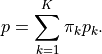
It represents the fact that a random variable $X$ can be seen as issued from one the $p_k$ , each with a probability $\pi_k$ . As a consequence, it is suitable for model-based clustering, where a cluster is a set of points issued from the same distribution $p_k$ , which is unknown, as $k$ is for a given point.

Note that there is a fundamental difference with Convolutions: in the latter, the random variable is a sum of random variables while in mixtures, the probability measure of the mixture random variable is a weighted sum of probability measures of random variables.

Constructor#

Mixtures are built from their components and weights:

>>> D1 = NegativeBinomial(0, 1, 0.1)
>>> D2 = Binomial(0, 10, 0.5)
>>> D3 = Binomial(1, 5, 0.2)
>>> M = Mixture(0.4, D1, 0.4, D2, 0.2, D3)

In order to display the contents, or to save the data, one uses methods Display() and plot().

Plotting#

>>> clf()
>>> import openalea.stat_tool.plot
>>> plot.DISABLE_PLOT=True
>>> print(M.display())
MIXTURE 3 DISTRIBUTIONS
mean: 5.93362   median: 4   mode: 2
variance: 42.8149   standard deviation: 6.54331   lower quartile: 2   upper quartile: 7

DISTRIBUTION 1 WEIGHT : 0.4
NEGATIVE_BINOMIAL   INF_BOUND : 0   PARAMETER : 1   PROBABILITY : 0.1
mean: 9   median: 6   mode: 0
variance: 90   standard deviation: 9.48683   lower quartile: 2   upper quartile: 13

DISTRIBUTION 2 WEIGHT : 0.4
BINOMIAL   INF_BOUND : 0   SUP_BOUND : 10   PROBABILITY : 0.5
mean: 5   median: 5   mode: 5
variance: 2.5   standard deviation: 1.58114   lower quartile: 4   upper quartile: 6

DISTRIBUTION 3 WEIGHT : 0.2
BINOMIAL   INF_BOUND : 1   SUP_BOUND : 5   PROBABILITY : 0.2
mean: 1.8   median: 2   mode: 1.5
variance: 0.64   standard deviation: 0.8   lower quartile: 1   upper quartile: 2

distances between components
          0.592991  0.6289
0.592991            0.800925
0.6289    0.800925

>>> M.plot()
>>> savefig('user/stat_tool_mixture1.png')

The following figure gathers the probability (mass) function, PMF, of the mixture and the weighted PMFs of its components.

Simulate#

Once you have a Mixture, you can simulate a data set using sample size as an argument:

>>> simulation = M.simulate(400)

This creates an Histogram, formally a openalea.stat_tool._stat_tool._DiscreteMixtureData that is associated with the mixture. Thus, plotting it provides both simulated data and distribution. Since in simulations, clusters are actually known at the time these are simulated, each component can be displayed separately:

>>> clf()
>>> simulation.plot()
>>> savefig('user/mixture_simul.png')

Estimate#

A Mixture can be estimated from a Histogram or a derived class, such as openalea.stat_tool._stat_tool._DiscreteMixtureData, using openalea.stat_tool.estimate.Estimate(). The parametric family of each component is passed as an argument in an abbreviated way: “B” for Binomial, “NB” for Negative Binomial, “P” for Poisson, etc.

>>> M_est = Estimate(simulation, "Mixture", "NB", "B", "B")
>>> print(M_est.display())
MIXTURE 3 DISTRIBUTIONS
mean: 5.52754   median: 4   mode: 2
variance: 32.6141   standard deviation: 5.71087   lower quartile: 2   upper quartile: 6

frequency distribution - sample size: 400
mean: 5.54   median: 4   mode: 1
variance: 33.1262   standard deviation: 5.75554   lower quartile: 2   upper quartile: 6

log-likelihood: -1060.51   (normalized: -2.65128)
maximum possible log-likelihood: -1040.61   (information: -2.60152)
deviance: 39.8066

11 free parameters   2 * penalyzed log-likelihood (AIC): -2143.03
11 free parameters   2 * penalyzed log-likelihood (AICc): -2143.71
11 free parameters   2 * penalyzed log-likelihood (BIC): -2186.93
11 free parameters   2 * penalyzed log-likelihood (BICc): -2175.93

log-likelihood for the optimal classification: -1171.28   (normalized: -2.92821)
maximum possible log-likelihood for the optimal classification: -1149.62   (information: -2.87406)

chi-square test (16 degrees of freedom)
chi-square value: 24.5417   critical probability: 0.0783223
reference chi-square value: 26.2962   reference critical probability: 0.05

DISTRIBUTION 1  WEIGHT : 0.137448
NEGATIVE_BINOMIAL   INF_BOUND : 0   PARAMETER : 9.32363   PROBABILITY : 0.351197
mean: 17.2245   median: 16   mode: 15
variance: 49.0452   standard deviation: 7.00323   lower quartile: 12   upper quartile: 21

frequency distribution 1 - sample size: 54
mean: 17.4815   median: 16.5   mode: 13
variance: 48.6317   standard deviation: 6.97365   lower quartile: 13   upper quartile: 22

DISTRIBUTION 2  WEIGHT : 0.415189
BINOMIAL   INF_BOUND : 0   SUP_BOUND : 8   PROBABILITY : 0.233856
mean: 1.87085   median: 2   mode: 2
variance: 1.43334   standard deviation: 1.19722   lower quartile: 1   upper quartile: 3

frequency distribution 2 - sample size: 167
mean: 1.86228   median: 2   mode: 1
variance: 1.38453   standard deviation: 1.17666   lower quartile: 1   upper quartile: 3

DISTRIBUTION 3  WEIGHT : 0.447363
BINOMIAL   INF_BOUND : 0   SUP_BOUND : 10   PROBABILITY : 0.533806
mean: 5.33806   median: 5   mode: 5
variance: 2.48857   standard deviation: 1.57752   lower quartile: 4   upper quartile: 6

frequency distribution 3 - sample size: 179
mean: 5.36872   median: 5   mode: 5
variance: 2.50373   standard deviation: 1.58232   lower quartile: 4   upper quartile: 7

distances between components
          0.976936  0.895427
0.976936            0.785317
0.895427  0.785317

Note that the order of the two Binomial components is arbitrary, thus they are likely to be switched.

Discrete mixtures of multivariate distributions#

Mixtures can be extended to multivariate distributions. The associated class is _MultivariateMixture, which works essentially as DiscreteMixture. Here is an example with 2 variables:

>>> from openalea.stat_tool.multivariate_mixture import _MultivariateMixture
>>>
>>> d11 = Binomial(0, 12, 0.1)
>>> d12 = Binomial(0, 12, 0.6)
>>> d13 = Binomial(0, 12, 0.9)
>>>
>>> d21 = Poisson(0, 25.0)
>>> d22 = Poisson(0, 5.0)
>>> d23 = Poisson(0, 0.2)
>>>
>>> m = _MultivariateMixture([0.1, 0.2, 0.7], [[d11, d21], [d12, d22], [d13, d23]])
>>> print(m)
MIXTURE

3 DISTRIBUTIONS

WEIGHTS
0.1  0.2  0.7

2 VARIABLES

VARIABLE 1 : DISCRETE_PARAMETRIC

STATE 0 OBSERVATION_DISTRIBUTION
BINOMIAL   INF_BOUND : 0   SUP_BOUND : 12   PROBABILITY : 0.1
mean: 1.2   median: 1   mode: 1
variance: 1.08   standard deviation: 1.03923   lower quartile: 0   upper quartile: 2

STATE 1 OBSERVATION_DISTRIBUTION
BINOMIAL   INF_BOUND : 0   SUP_BOUND : 12   PROBABILITY : 0.6
mean: 7.2   median: 7   mode: 7
variance: 2.88   standard deviation: 1.69706   lower quartile: 6   upper quartile: 8

STATE 2 OBSERVATION_DISTRIBUTION
BINOMIAL   INF_BOUND : 0   SUP_BOUND : 12   PROBABILITY : 0.9
mean: 10.8   median: 11   mode: 11
variance: 1.08   standard deviation: 1.03923   lower quartile: 10   upper quartile: 12

VARIABLE 2 : DISCRETE_PARAMETRIC

STATE 0 OBSERVATION_DISTRIBUTION
POISSON   INF_BOUND : 0   PARAMETER : 25
mean: 25   median: 25   mode: 24.5
variance: 25   standard deviation: 5   lower quartile: 22   upper quartile: 28

STATE 1 OBSERVATION_DISTRIBUTION
POISSON   INF_BOUND : 0   PARAMETER : 5
mean: 5   median: 5   mode: 4.5
variance: 5   standard deviation: 2.23607   lower quartile: 3   upper quartile: 6

STATE 2 OBSERVATION_DISTRIBUTION
POISSON   INF_BOUND : 0   PARAMETER : 0.2
mean: 0.2   median: 0   mode: 0
variance: 0.2   standard deviation: 0.447214   lower quartile: 0   upper quartile: 0

The Plot function plots the mixture marginals:

>>> Plot(m, Title="Mixture model used for simulation: ")

Marginals can also be extracted as distributions:

>>> marg1 = m.extract_mixture(1) # first variable
>>> print(marg1)
coefficient of concentration: 0.177522 | 0.177522
CATEGORICAL
mean: 9.12   median: 10   mode: 11
variance: 10.4256   standard deviation: 3.22887   lower quartile: 8   upper quartile: 11
coefficient of skewness: -1.49966   coefficient of kurtosis: 1.32361
mean absolute deviation: 2.45149   coefficient of concentration: 0.177522
information: -2.11067

Vectors can be simulated with openalea.stat_tool._stat_tool._MultivariateMixture.simulate():

>>> print("Simulate multivariate mixture: ")
Simulate multivariate mixture:
>>> set_seed(1)
>>> v = m.simulate(500000)

Multivariate mixtures can be estimated by the EM algorithm from Vectors with openalea.stat_tool._stat_tool._MultivariateMixtureData.mixture_estimation():

>>> m_estim_model = v.mixture_estimation(m, 100,  [True, True])
>>> print(m_estim_model)
MIXTURE

3 DISTRIBUTIONS

WEIGHTS
0.0999758  0.20025  0.699774

2 VARIABLES

VARIABLE 1 : DISCRETE_PARAMETRIC


STATE 0 OBSERVATION_DISTRIBUTION
BINOMIAL   INF_BOUND : 0   SUP_BOUND : 12   PROBABILITY : 0.0999885
mean: 1.19986   median: 1   mode: 1
variance: 1.07989   standard deviation: 1.03918   lower quartile: 0   upper quartile: 2

state 0 observation frequency distribution - sample size: 49989
mean: 1.19982   median: 1   mode: 1
variance: 1.08568   standard deviation: 1.04196   lower quartile: 0   upper quartile: 2

STATE 1 OBSERVATION_DISTRIBUTION
BINOMIAL   INF_BOUND : 0   SUP_BOUND : 12   PROBABILITY : 0.600068
mean: 7.20081   median: 7   mode: 7
variance: 2.87984   standard deviation: 1.69701   lower quartile: 6   upper quartile: 8

state 1 observation frequency distribution - sample size: 98510
mean: 7.16891   median: 7   mode: 7
variance: 2.83682   standard deviation: 1.68429   lower quartile: 6   upper quartile: 8

STATE 2 OBSERVATION_DISTRIBUTION
BINOMIAL   INF_BOUND : 0   SUP_BOUND : 12   PROBABILITY : 0.900095
mean: 10.8011   median: 11   mode: 11
variance: 1.07909   standard deviation: 1.03879   lower quartile: 10   upper quartile: 12

state 2 observation frequency distribution - sample size: 351501
mean: 10.7936   median: 11   mode: 11
variance: 1.095   standard deviation: 1.04642   lower quartile: 10   upper quartile: 12

VARIABLE 2 : DISCRETE_PARAMETRIC


STATE 0 OBSERVATION_DISTRIBUTION
POISSON   INF_BOUND : 0   PARAMETER : 25.0277
mean: 25.0277   median: 25   mode: 25
variance: 25.0277   standard deviation: 5.00277   lower quartile: 22   upper quartile: 28

state 0 observation frequency distribution - sample size: 49989
mean: 25.0282   median: 25   mode: 24
variance: 24.859   standard deviation: 4.98588   lower quartile: 22   upper quartile: 28

STATE 1 OBSERVATION_DISTRIBUTION
POISSON   INF_BOUND : 0   PARAMETER : 5.00441
mean: 5.00441   median: 5   mode: 5
variance: 5.00441   standard deviation: 2.23705   lower quartile: 3   upper quartile: 6

state 1 observation frequency distribution - sample size: 98510
mean: 5.0797   median: 5   mode: 5
variance: 4.68722   standard deviation: 2.165   lower quartile: 3   upper quartile: 6

STATE 2 OBSERVATION_DISTRIBUTION
POISSON   INF_BOUND : 0   PARAMETER : 0.19947
mean: 0.19947   median: 0   mode: 0
variance: 0.19947   standard deviation: 0.446621   lower quartile: 0   upper quartile: 0

state 2 observation frequency distribution - sample size: 351501
mean: 0.200301   median: 0   mode: 0
variance: 0.195032   standard deviation: 0.441624   lower quartile: 0   upper quartile: 0

information: -1e+37 (-2e+31)

log-likelihood: -1.69433e+06   (normalized: -3.38866)
deviance: -2e+37

17 free parameters   2 * penalyzed log-likelihood (AIC): -3.38869e+06
17 free parameters   2 * penalyzed log-likelihood (AICc): -3.38869e+06
17 free parameters   2 * penalyzed log-likelihood (BIC): -3.38888e+06
17 free parameters   2 * penalyzed log-likelihood (BICc): -3.38886e+06