Operations on data with stat_tool#

This notebook illustates how to perform basic operations on data with stat_tool.data_transform#

The main data structures in stat_tool are Vectors and Histogram. Histogram is basically a 1-D array or a multiset of integers. Possibilities are offered of combining histograms with Merge, adding constants to values with Shift, filtering values with ValueSelect and renaming values with Transcode.

The specificity of Vectors are the presence of several variables: the additional possible operations with respect to Histogram are merging variables .

Transform data on Vectors#

We first load a data set (chene_sessile.vec)

[1]:

from openalea.stat_tool import (get_shared_data,
                                Histogram
)
from openalea.stat_tool.data_transform import (SelectVariable,
                                               SelectIndividual,
                                               Merge,
                                               MergeVariable,
                                               Shift,
                                               ValueSelect
)
from openalea.stat_tool.output import Plot
from openalea.stat_tool.vectors import Vectors
from openalea.stat_tool.cluster import Transcode

vec = Vectors(get_shared_data("chene_sessile.vec"))

Running cmake --build & --install in /home/jdurand/devlp/Git/openalea/stat_tool/build
Running cmake --build & --install in /home/jdurand/devlp/Git/openalea/sequence_analysis/build

[2]:

print(vec)

138 vectors

6 VARIABLES

VARIABLE 1 : INT   (minimum value: 1995, maximum value: 1997)

marginal frequency distribution - sample size: 138
mean: 1996   median: 1996   mode: 1996
variance: 0.671533   standard deviation: 0.819471   lower quartile: 1995   upper quartile: 1997

VARIABLE 2 : INT   (minimum value: 4, maximum value: 110)

marginal frequency distribution - sample size: 138
mean: 42.8043   median: 37   mode: 26
variance: 539.064   standard deviation: 23.2177   lower quartile: 24   upper quartile: 61

VARIABLE 3 : INT   (minimum value: 39, maximum value: 219)

marginal frequency distribution - sample size: 138
mean: 107.725   median: 102   mode: 85
variance: 1424.04   standard deviation: 37.7365   lower quartile: 84   upper quartile: 131

VARIABLE 4 : INT   (minimum value: 1, maximum value: 4)

marginal frequency distribution - sample size: 138
mean: 1.63768   median: 2   mode: 2
variance: 0.349519   standard deviation: 0.591201   lower quartile: 1   upper quartile: 2

   | frequency
0   0
1  57
2  75
3   5
4   1

VARIABLE 5 : INT   (minimum value: 8, maximum value: 63)

marginal frequency distribution - sample size: 138
mean: 30.9783   median: 28   mode: 33
variance: 179.934   standard deviation: 13.4139   lower quartile: 21   upper quartile: 40

VARIABLE 6 : INT   (minimum value: 0, maximum value: 19)

marginal frequency distribution - sample size: 138
mean: 5.19565   median: 5   mode: 0
variance: 21.341   standard deviation: 4.61963   lower quartile: 1   upper quartile: 8

correlation matrix

           1          2          3          4          5          6
1          1  -0.223663   -0.75155  -0.316395  -0.258309  -0.775112
2  -0.223663          1   0.557942   0.649939   0.883212   0.386496
3   -0.75155   0.557942          1   0.446346   0.501469   0.693231
4  -0.316395   0.649939   0.446346          1   0.681954   0.378931
5  -0.258309   0.883212   0.501469   0.681954          1   0.425416
6  -0.775112   0.386496   0.693231   0.378931   0.425416          1

reference t-value: 1.97756   reference critical probability: 0.05
limit correlation coefficient: 0.167188

reference t-value: 2.61246   reference critical probability: 0.01
limit correlation coefficient: 0.218599

Note that vec2 contains 6 variables.

Selecting variables#

We can select the first two variables using function SelectVariable:

[3]:

vec2 = SelectVariable(vec, [1,2], "Keep")

This is equivalent to using the method Vectors.select_variable, except that the last argument is Keep in [True, False] instead of Mode in [“Keep”, “Reject”].

[4]:

assert(str(vec2) == str(vec.select_variable([1,2], True)))

We can check that only 2 variables are remaining:

[5]:

vec2.nb_variable

[5]:

Setting argument “Keep” to False would discard variables [1,2]:

[6]:

assert(vec.select_variable([1,2], False).nb_variable == 4)

Selecting individuals#

In the same way we can select variables, we can also select individuals:

[7]:

subvec = SelectIndividual(vec,list(range(30, 120)), "Keep")

…which is equivalent to

[8]:

assert(str(subvec) == str(vec.select_individual(list(range(30, 120)), True)))

Merging Vectors#

Vectors with the same dimension can be merged (individual-wise):

[9]:

vec_i1 = Vectors([[0, 0, 0], [1, 1, 1]])
vec_i2 = Vectors([[2, 2, 2], [3, 3, 3]])
vec_i3 = Vectors([[4, 4, 4]])
vec_merged = Merge(vec_i1, vec_i2, vec_i3)
vec_merged.nb_vector

[9]:

This is equivalent to using the method Vectors.merge:

[10]:

str(vec_i1.merge([vec_i2, vec_i3])) == str(vec_merged)

[10]:

True

[11]:

print(vec_merged[4])

[4, 4, 4]

It can be seen that the last vector from the merge Vectors is the last vector from vec_i3.

Similarly, Vectors with the same numbers of individuals can be merged (variable-wise):

[12]:

vec_v2 = Vectors([[5], [5], [5], [5], [5]])
vec_vmerged = MergeVariable(vec_merged, vec_v2, RefSample=1)

The RefSample argument is optional here and is used only to give identifiers to vectors using one of the samples as a reference, here sample 1.

[13]:

print(vec_vmerged[0])

[0, 0, 0, 5]

It can be seen that the variable from vec_v2 has been added to the 3 variables from vec_merged.

This is equivalent to using the method Vectors.merge_variable:

[14]:

print((vec_merged.merge_variable([vec_v2],1))[0])

[0, 0, 0, 5]

Shifting Vectors#

Shifting a vector is the operation consisting in adding a constant to each value of a variable:

[15]:

print(vec2)

138 vectors

2 VARIABLES

VARIABLE 1 : INT   (minimum value: 1995, maximum value: 1997)

marginal frequency distribution - sample size: 138
mean: 1996   median: 1996   mode: 1996
variance: 0.671533   standard deviation: 0.819471   lower quartile: 1995   upper quartile: 1997

VARIABLE 2 : INT   (minimum value: 4, maximum value: 110)

marginal frequency distribution - sample size: 138
mean: 42.8043   median: 37   mode: 26
variance: 539.064   standard deviation: 23.2177   lower quartile: 24   upper quartile: 61

correlation matrix

           1          2
1          1  -0.223663
2  -0.223663          1

reference t-value: 1.97756   reference critical probability: 0.05
limit correlation coefficient: 0.167188

reference t-value: 2.61246   reference critical probability: 0.01
limit correlation coefficient: 0.218599

[16]:

print(Shift(vec2, 1, 2))

138 vectors

2 VARIABLES

VARIABLE 1 : INT   (minimum value: 1997, maximum value: 1999)

marginal frequency distribution - sample size: 138
mean: 1998   median: 1998   mode: 1998
variance: 0.671533   standard deviation: 0.819471   lower quartile: 1997   upper quartile: 1999

VARIABLE 2 : INT   (minimum value: 4, maximum value: 110)

marginal frequency distribution - sample size: 138
mean: 42.8043   median: 37   mode: 26
variance: 539.064   standard deviation: 23.2177   lower quartile: 24   upper quartile: 61

correlation matrix

           1          2
1          1  -0.223663
2  -0.223663          1

reference t-value: 1.97756   reference critical probability: 0.05
limit correlation coefficient: 0.167188

reference t-value: 2.61246   reference critical probability: 0.01
limit correlation coefficient: 0.218599

Here, variable 1 (second argument) has been shifted by 2 (third argument).

If a Vectors object has only one variable, the variable does not have to be passed as an argument:

[17]:

Shift(vec_v2, 2)[0]

[17]:

[7]

As usual, it is equivalent to use method Vectors.shift:

[18]:

print([vec2.get_min_value(0), vec2.shift(1, 2).get_min_value(0)])

[1995.0, 1997.0]

Vectors can be shifted by negative values:

[19]:

Shift(vec_i2, 1, -3)[0]

[19]:

[-1, 2, 2]

### Selecting individuals by values (filtering individuals)

Individual vectors in Vectors can be selected or discarded according to their values.

For example,

[20]:

ValueSelect(vec_merged, 1, 2, 3).nb_vector

[20]:

selects all vectors in vec_merged such that variable 1 is between 2 and 3.

To discard all such vectors, use argument ‘Mode = “Reject”’:

[21]:

ValueSelect(vec_merged, 1, 2, 3, Mode="Reject").nb_vector

[21]:

The object-oriented syntax is:

[22]:

vec_merged.value_select(1, 2, 3, True)

[22]:

<openalea.stat_tool._stat_tool._Vectors at 0x783e4022c9e0>

where the last argument corresponds to ‘Keep=True’.

Transcoding Vectors#

Transcoding the values of a Vectors object consists in replacing a value by another one. To use function Transcode, the list of values that replace the former ones is placed as argument:

[23]:

Transcode(vec_merged, 1, [0, -1, -2, -3, -4])

[23]:

<openalea.stat_tool._stat_tool._Vectors at 0x783e4022c900>

This is equivalent to using method Vectors.transcode:

[24]:

print([vec_merged.transcode(1, [0, -1, -2, -3, -4])[i][0] for i in range(vec_merged.nb_vector)])

[0, -1, -2, -3, -4]

[25]:

print([vec_merged[i][0] for i in range(vec_merged.nb_vector)])

[0, 1, 2, 3, 4]

Note that 0 has been replaced by 0, 1 by -1, etc.

Transform data on Histograms#

Merging histograms#

Histogram objects can be merged, which consists in adding counts of each histogram.

It can be seen from y-axis in the last figure that counts match the sum of counts of the 2 previous figures.

[26]:

meri1 = Histogram(get_shared_data("meri1.his"))
meri2 = Histogram(get_shared_data("meri2.his"))
meri12 = Merge(meri1, meri2)

[27]:

Plot(meri1)
Plot(meri2)
Plot(meri12)

../_images/examples_data_transform_65_0.png

../_images/examples_data_transform_65_1.png

../_images/examples_data_transform_65_2.png

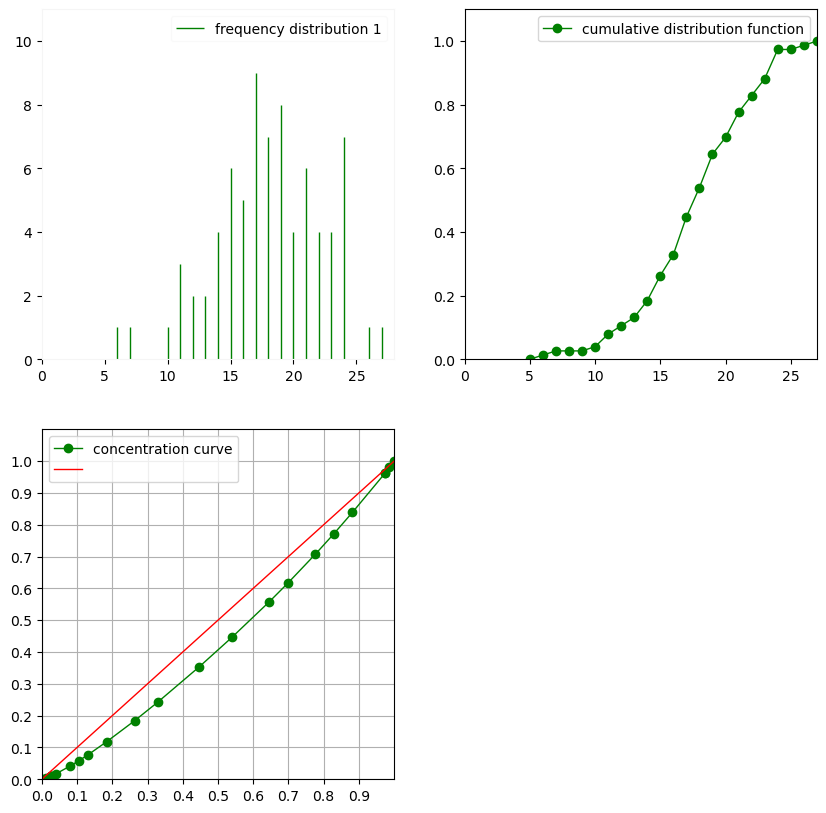
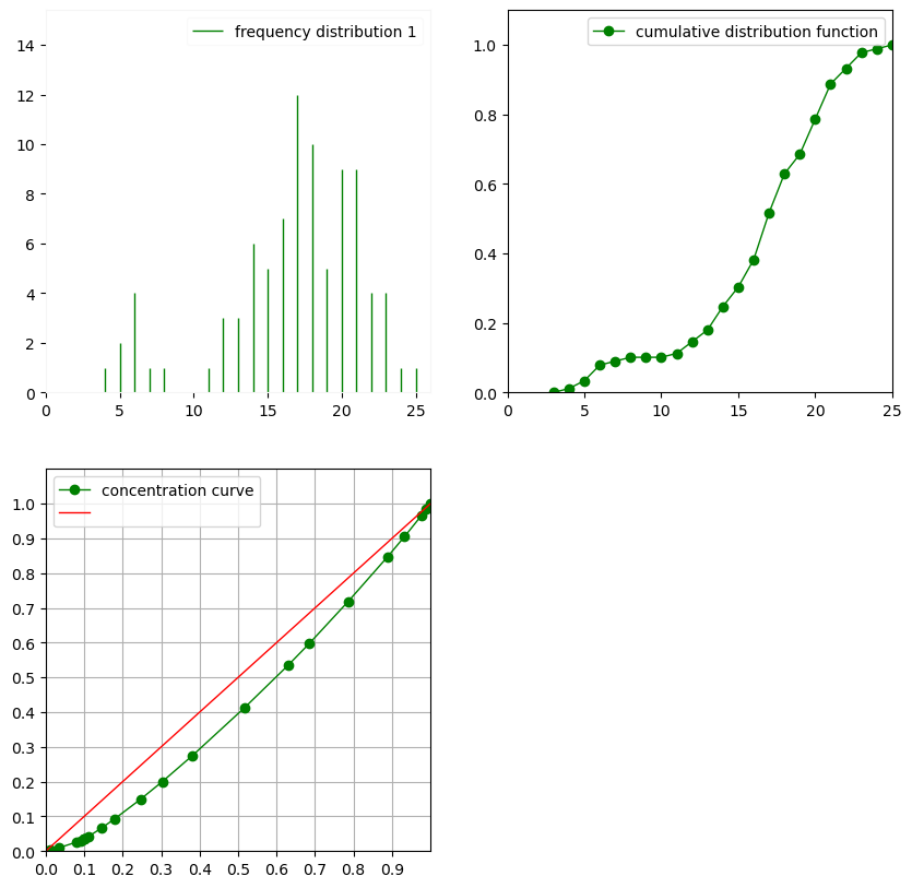
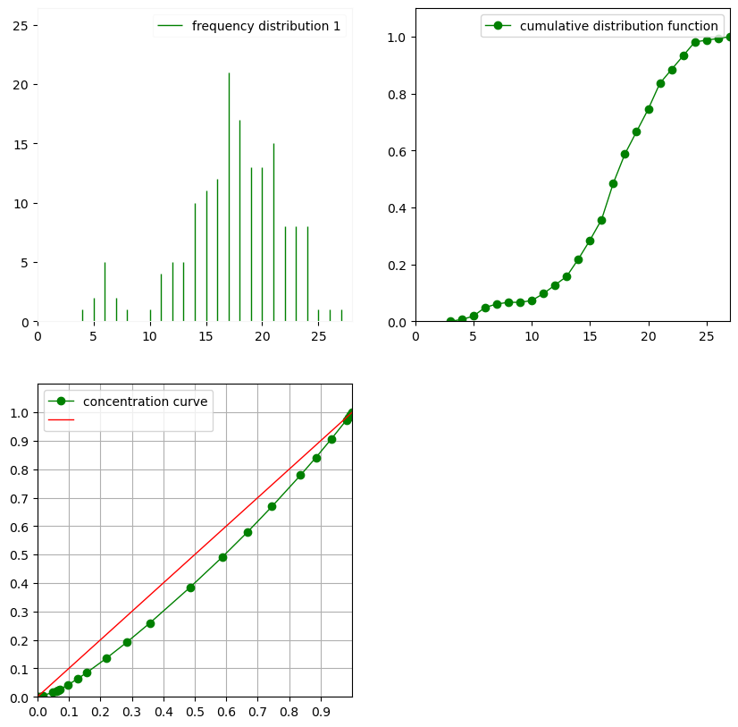
Arbitrary numbers of Histogram objects can be merged:

[28]:

meri3 = Histogram(get_shared_data("meri3.his"))
meri123 = Merge(meri1, meri2, meri3)

This is equivalent to the method Histogram.merge:

[29]:

meri123b = meri1.merge([meri2, meri3])
assert(str(meri123) == str(meri123b))

Shifting histograms#

As Vectors, Histogram objects can be shifted:

[30]:

Plot(meri1)
Plot(Shift(meri1,3))

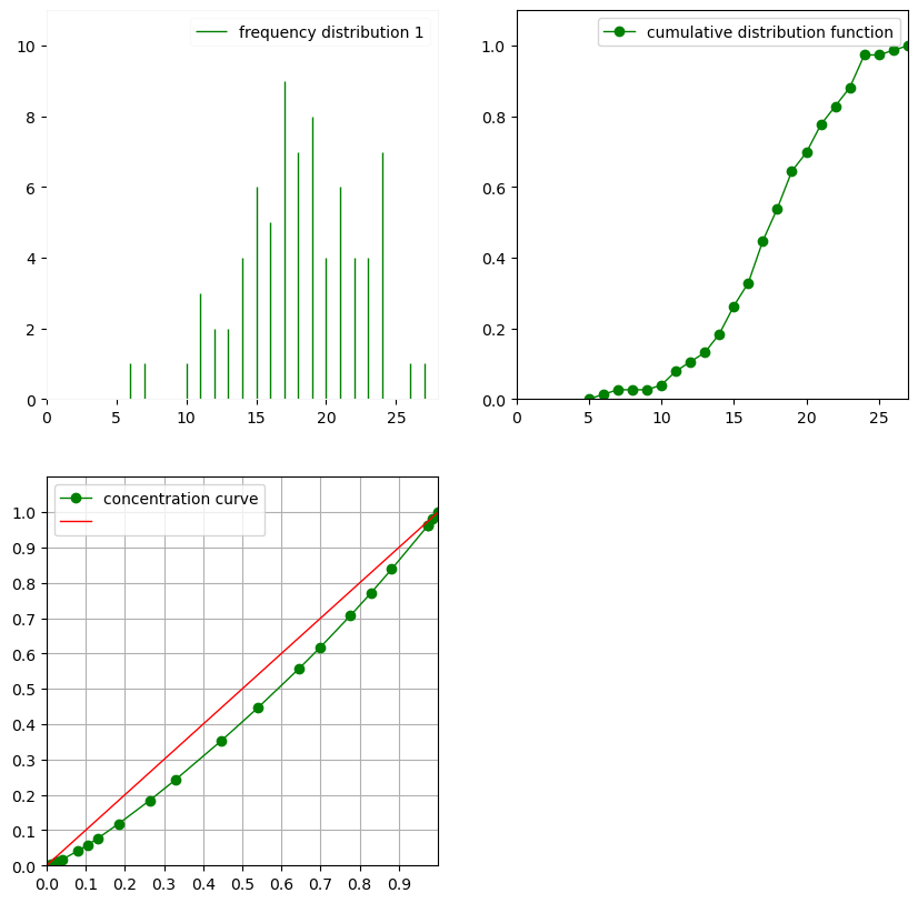
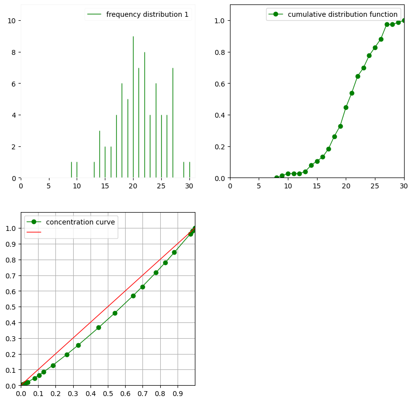
../_images/examples_data_transform_72_0.png

../_images/examples_data_transform_72_1.png

All values have been shifted by 3 (shift of the x-axis). This is equivalent to Histogram.shift:

[31]:

assert(str(Shift(meri1,3)) == str(meri1.shift(3)))

### Selecting individuals by values (filtering histograms)

As Vectors, Histogram objects can be filtered:

[32]:

Plot(meri1)
Plot(ValueSelect(meri1,15,25))

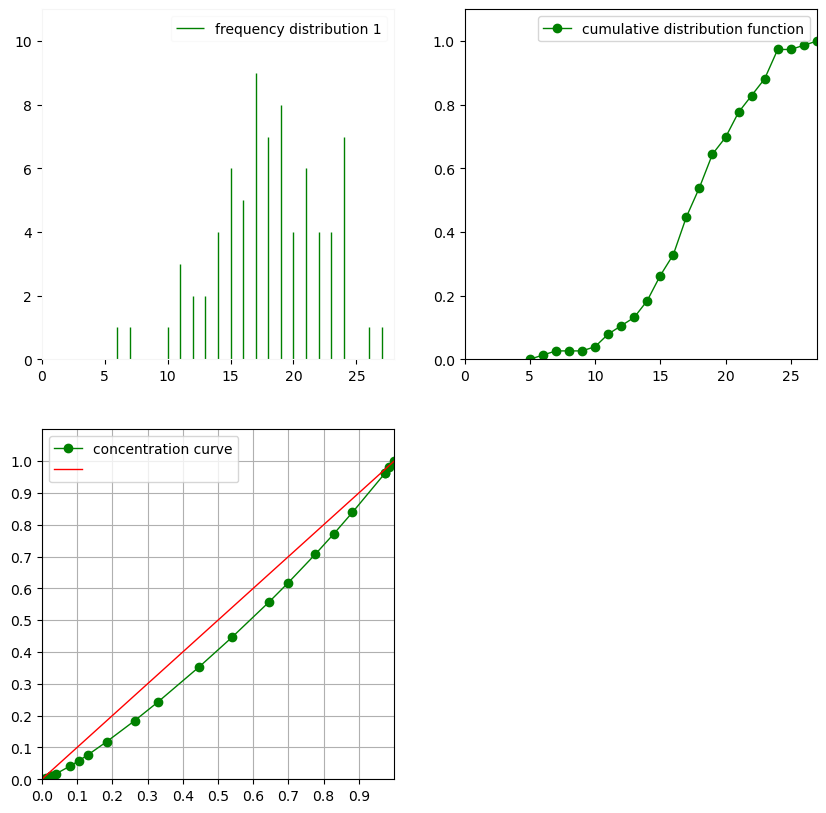
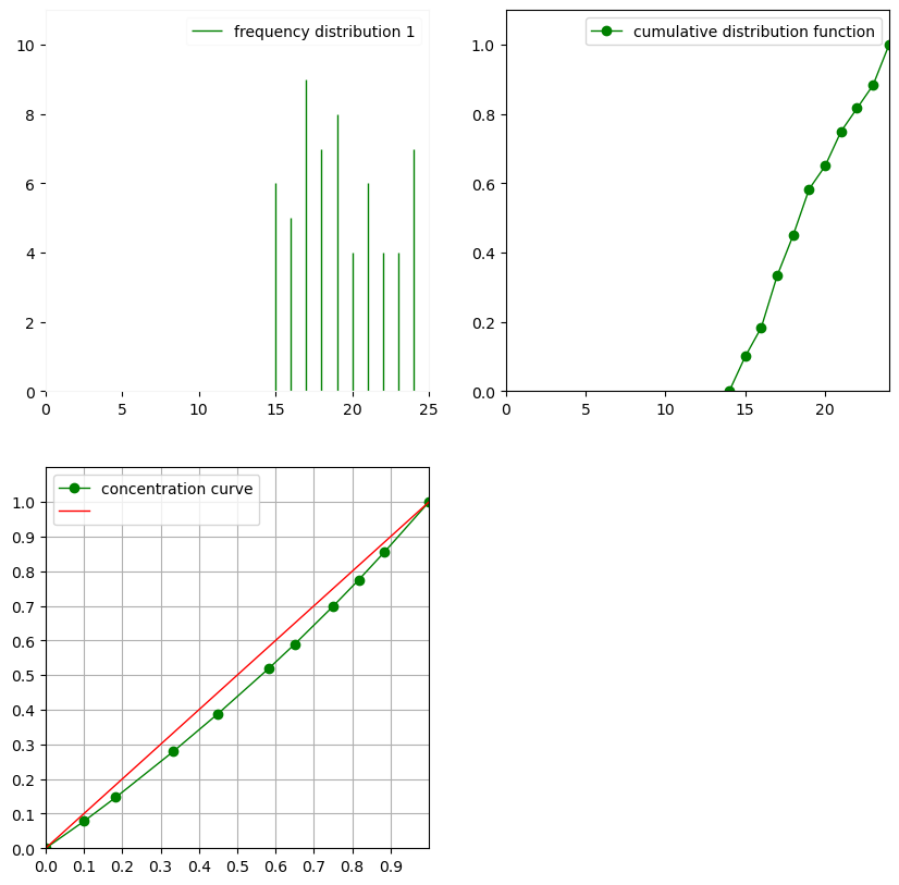
../_images/examples_data_transform_77_0.png

../_images/examples_data_transform_77_1.png

Here, only the values between 15 and 25 have been selected. This is equivalent with Histogram.value_select

[33]:

assert(str(ValueSelect(meri1,15,25)) == str(meri1.value_select(15,25,True)))

Transcoding Histograms#

As Vectors, the values of Histogram objects can be transcoded.

Note that:

The first successive values in the range of the Histogram with null frequencies (range(0, Histogram.offset-1)) do not count, they cannot be transcoded.
The other values with null frequencies do count, they are include in the list defining transcoding.

Here, to simplify the example, we restrict the Histogram to values 6, 7, 8, 9, 10.

[34]:

meri_vselect = ValueSelect(meri1,6,10)
print(meri_vselect.display(Detail=2))

frequency distribution - sample size: 3
mean: 7.66667   median: 7   mode: 6.5
variance: 4.33333   standard deviation: 2.08167   lower quartile: 6   upper quartile: 10
coefficient of skewness: 1.29334   coefficient of kurtosis: -2
mean absolute deviation: 1.55556   coefficient of concentration: 0.115942
information: -3.29584 (-1.09861)

   | frequency distribution | cumulative distribution function
 0  0         0
 1  0         0
 2  0         0
 3  0         0
 4  0         0
 5  0         0
 6  1  0.333333
 7  1  0.666667
 8  0  0.666667
 9  0  0.666667
10  1         1

[35]:

range(0, meri_vselect.offset-1)

[35]:

range(0, 5)

The transcoding is

$6 \rightarrow 2$
$7 \rightarrow 4$
$8 \rightarrow 1$
$9 \rightarrow 3$
$10 \rightarrow 0$

[36]:

meri_transcoded = Transcode(meri_vselect,[2, 4, 1, 3, 0])
print(meri_transcoded.display(Detail=2))

frequency distribution - sample size: 3
mean: 2   median: 2   mode: 0
variance: 4   standard deviation: 2   lower quartile: 0   upper quartile: 4
coefficient of skewness: 0   coefficient of kurtosis: -2
mean absolute deviation: 1.33333   coefficient of concentration: 0.444444
information: -3.29584 (-1.09861)

   | frequency distribution | cumulative distribution function
0  1  0.333333
1  0  0.333333
2  1  0.666667
3  0  0.666667
4  1         1